Getting State & County Boundaries
Objectives:
- Use {
USAboundaries} package to download and save boundary data for State and Counties - save out data in different spatial formats: (
.shp,.geojson,.kml,.csv)
Downloading US Boundaries
There are several options to do this, and many work equally well. We’ll demonstrate one possible option here, the USAboundaries package.
Loading Spatial Packages
Make sure you load the following packages
# load packages or "libraries"
library(tidyverse) # wrangling/plotting tools
library(sf) # "simple features" spatial package for vector based data
library(USAboundaries) # data for USA boundaries
Get State Boundary Data
Now lets grab some data using a package called USAboundaries, which allows us to quickly download county or state outlines, in sf formats. Very handy for making some quick professional maps.
First we’ll grab a State boundary for CA, OR, and NV so we can filter these down later.
library(USAboundaries)

# Pick a State
state_names <- c("california", "oregon", "nevada") # a vector of names

# Download STATE data and add projection
states <- us_states(resolution = "high", states = state_names) # what does resolution do?

st_crs(states) # double check the CRS
## Coordinate Reference System:
## User input: EPSG:4326
## wkt:
## GEOGCRS["WGS 84",
## DATUM["World Geodetic System 1984",
## ELLIPSOID["WGS 84",6378137,298.257223563,
## LENGTHUNIT["metre",1]]],
## PRIMEM["Greenwich",0,
## ANGLEUNIT["degree",0.0174532925199433]],
## CS[ellipsoidal,2],
## AXIS["geodetic latitude (Lat)",north,
## ORDER[1],
## ANGLEUNIT["degree",0.0174532925199433]],
## AXIS["geodetic longitude (Lon)",east,
## ORDER[2],
## ANGLEUNIT["degree",0.0174532925199433]],
## USAGE[
## SCOPE["unknown"],
## AREA["World"],
## BBOX[-90,-180,90,180]],
## ID["EPSG",4326]]# make a quick plot!
plot(states$geometry)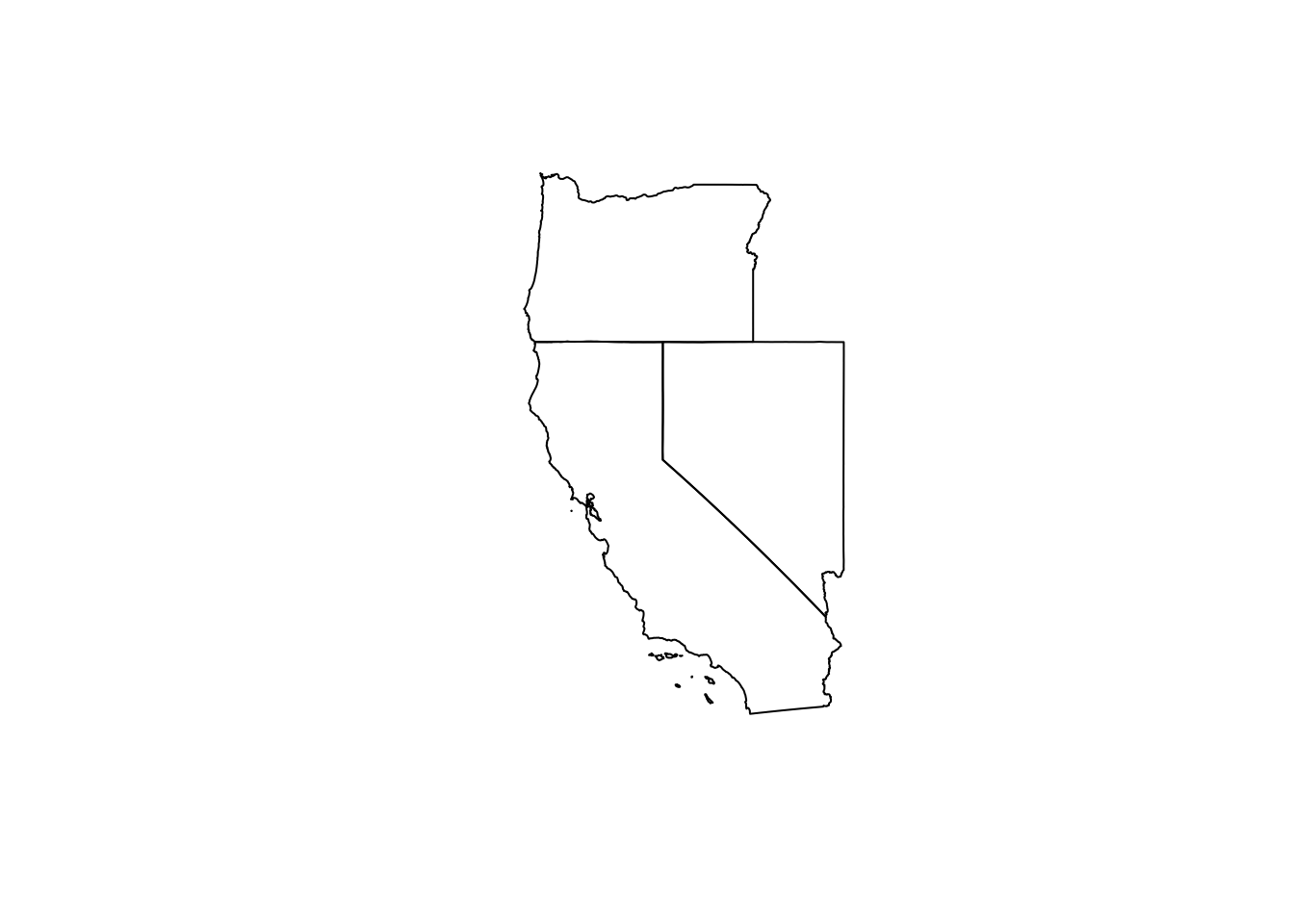
Save as .shp
A commonly used geospatial file format is the shapefile. Unfortunately this file type usually contains 4-5 or more associated files for each spatial object. So, when saving out as .shp, expect to see at least 4 files with the same name but different file extensions. All will be needed to spatially orient and read the data back in.
# save out as "shp"
st_write(states, "data/states_boundaries.shp",
         delete_dsn = TRUE) # setting to TRUE allows overwrite
## Warning in abbreviate_shapefile_names(obj): Field names abbreviated for ESRI Shapefile driver## Deleting source `data/states_boundaries.shp' using driver `ESRI Shapefile'
## Writing layer `states_boundaries' to data source `data/states_boundaries.shp' using driver `ESRI Shapefile'
## Writing 3 features with 12 fields and geometry type Multi Polygon.## Warning in CPL_write_ogr(obj, dsn, layer, driver, as.character(dataset_options), : GDAL Message 1: Value 403501101370 of field aland of feature 0 not
## successfully written. Possibly due to too larger number with respect to field width## Warning in CPL_write_ogr(obj, dsn, layer, driver, as.character(dataset_options), : GDAL Message 1: Value 20466718403 of field awater of feature 0 not
## successfully written. Possibly due to too larger number with respect to field width## Warning in CPL_write_ogr(obj, dsn, layer, driver, as.character(dataset_options), : GDAL Message 1: Value 284329326845 of field aland of feature 1 not
## successfully written. Possibly due to too larger number with respect to field width## Warning in CPL_write_ogr(obj, dsn, layer, driver, as.character(dataset_options), : GDAL Message 1: Value 2047350887 of field awater of feature 1 not
## successfully written. Possibly due to too larger number with respect to field width## Warning in CPL_write_ogr(obj, dsn, layer, driver, as.character(dataset_options), : GDAL Message 1: Value 248604268242 of field aland of feature 2 not
## successfully written. Possibly due to too larger number with respect to field width## Warning in CPL_write_ogr(obj, dsn, layer, driver, as.character(dataset_options), : GDAL Message 1: Value 6195105690 of field awater of feature 2 not
## successfully written. Possibly due to too larger number with respect to field widthSave as .kml
kml or Keyhole Markup Language is an XML format which is used by Google Earth and other programs. It can contain multiple layers (similar to .gpx), and retains the CRS associated with the data. Here we are writing a single layer (our states). But we could easily add (or append=TRUE) additional data like points or lines to this same file.
# save out as "kml"
st_write(states, "data/states_boundaries.kml",
         delete_dsn = TRUE) # setting to TRUE allows overwrite
## Deleting source `data/states_boundaries.kml' using driver `KML'
## Writing layer `states_boundaries' to data source `data/states_boundaries.kml' using driver `KML'
## Writing 3 features with 12 fields and geometry type Multi Polygon.# to read it back in...
states <- st_read("data/states_boundaries.kml")## Reading layer `states_boundaries' from data source `/Users/ryanpeek/Documents/github/TEACHING/2020_CABW_R_training/data/states_boundaries.kml' using driver `KML'
## Simple feature collection with 3 features and 2 fields
## geometry type: MULTIPOLYGON
## dimension: XY
## bbox: xmin: -124.5662 ymin: 32.53416 xmax: -114.0396 ymax: 46.29204
## geographic CRS: WGS 84Get County Boundaries
Let’s get counties for all of California, and then filter to a single county. Notice we give the us_counties function only one state, but could easily pass a vector of states as we did in the section above.
# Download outlines of all the counties for California
ca_counties<-us_counties(resolution = "high", states = "CA")

# Pick a county of interest
#co_names <- c("El Dorado")

# filter to just that county:
#eldor_co <- filter(ca_counties, name==co_names)

# save out
#st_write(eldor_co, "data/eldorado_county_boundary.shp")
Save as .geojson
An open source file type that requires a single file, is compatible with vector data, and is based on JSON. There are other packages that can be used to read/write these files, but we’ll stick with sf here.
st_write(ca_counties, "data/ca_counties_boundaries.geojson",
         delete_dsn = TRUE)
## Deleting source `data/ca_counties_boundaries.geojson' using driver `GeoJSON'
## Writing layer `ca_counties_boundaries' to data source `data/ca_counties_boundaries.geojson' using driver `GeoJSON'
## Writing 58 features with 12 fields and geometry type Multi Polygon.Save as .csv
We can always fall back on writing to a comma-delimited file, but with the inclusion of a geometry column as WKT (Well-known-text). This means the spatial data is written into the .csv, and then will need to be read in as such. Note, this format has a smaller file size compared with geojson and is comparable to .kml.
One downside is typically the CRS information isn’t retained in the csv, so you need to know what CRS the data has and then set the CRS using st_set_crs
# This writes the geometry column as a WKT (all in one column)
st_write(ca_counties, "data/ca_counties_boundaries.csv",
         layer_options = "GEOMETRY=AS_WKT",
         delete_dsn = TRUE)
## Deleting source `data/ca_counties_boundaries.csv' using driver `CSV'
## Writing layer `ca_counties_boundaries' to data source `data/ca_counties_boundaries.csv' using driver `CSV'
## options: GEOMETRY=AS_WKT
## Writing 58 features with 12 fields and geometry type Multi Polygon.# to read in:
ca_counties2 <- st_read("data/ca_counties_boundaries.csv",
stringsAsFactors = FALSE,
as_tibble = TRUE,
options="GEOM_POSSIBLE_NAMES=WKT") %>%
# drop the WKT column
dplyr::select(-WKT)## options: GEOM_POSSIBLE_NAMES=WKT
## Reading layer `ca_counties_boundaries' from data source `/Users/ryanpeek/Documents/github/TEACHING/2020_CABW_R_training/data/ca_counties_boundaries.csv' using driver `CSV'
## Simple feature collection with 58 features and 13 fields
## geometry type: MULTIPOLYGON
## dimension: XY
## bbox: xmin: -124.4096 ymin: 32.53416 xmax: -114.1312 ymax: 42.00952
## CRS: NA# also need to set the CRS:
ca_counties2 <- st_set_crs(ca_counties2, 4326)Make sure this all worked by previewing with tmap.
library(tmap)
tmap_mode(mode = "view")

tmap::tm_shape(ca_counties2) +
  tm_polygons(alpha=0.1, col="seagreen") +
  tm_shape(states) +
  tm_polygons(lwd=2, border.col = "gray10", alpha = 0, col=NA)