Spreadsheet to R
Objectives for this section:
- look at a messy spreadsheet & understand how to make it tidy
- read (import) data into R from different spreadsheet tabs
- write data to a
.xlsxspreadsheet, or a standalone.csv!
Spreadsheet Madness to Tidy Data
Spreadsheets surround us and exist in nearly every facet and field. While learning how to use will make life easier and more reproducible, spreadsheets won’t go away, and there will always still be a messy dataset that comes your way.
So let’s talk about what tidy data should look like, and then take a look at a messy real-life spreadsheet, and figure out what could be done to make it tidy!

Figure 1: Illustration by @allison_horst, from Hadley Wickham’s talk “The Joy of Functional Programming (for Data Science)”
What is Tidy Data?
Typically when we look at data, we should always want it to be in a “tidy” format. To be in a tidy format, we want to have each column as a unique variable, and each row as a unique observation of data.
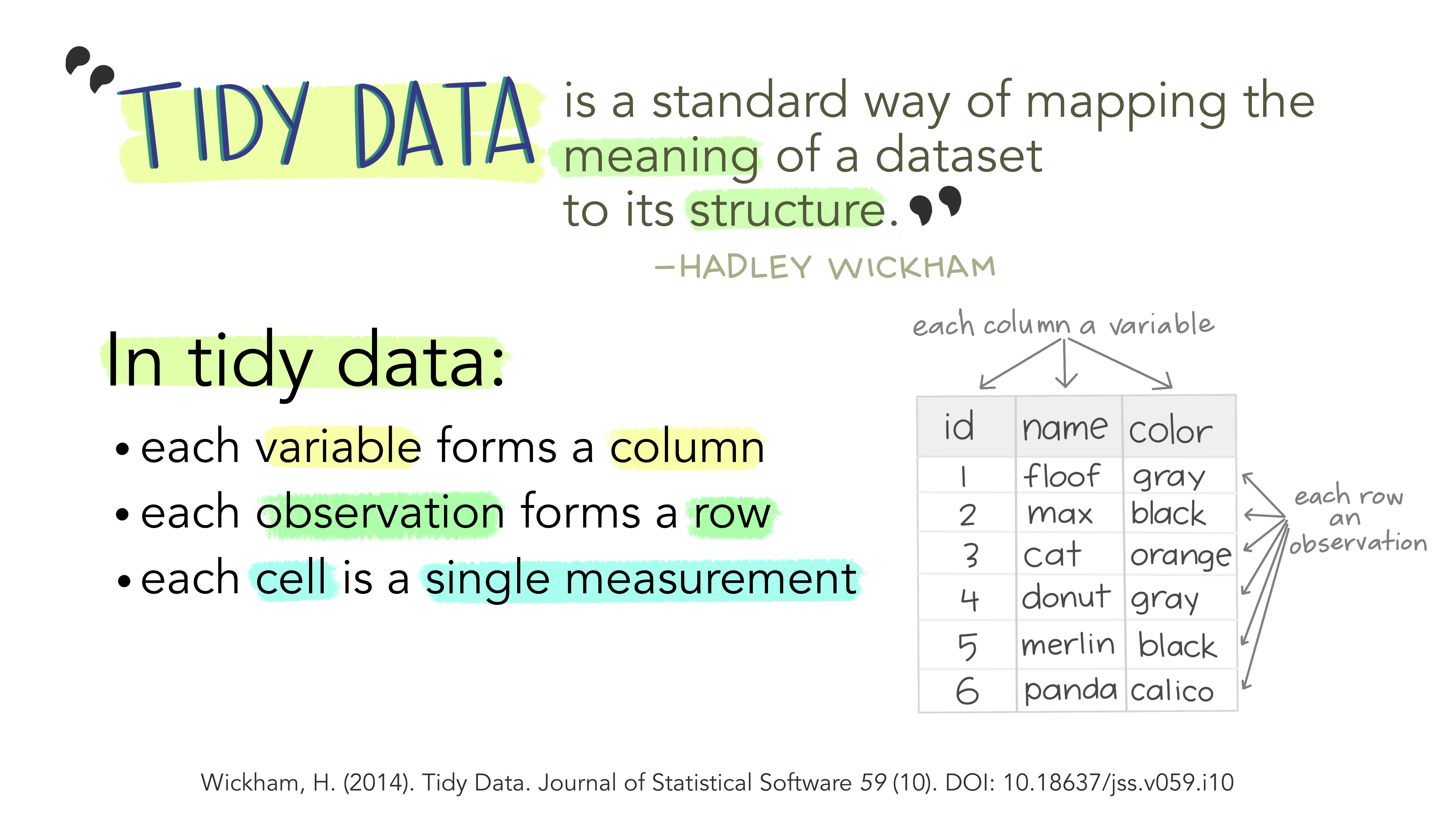
Figure 2: Illustrations from the Openscapes blog Tidy Data for reproducibility, efficiency, and collaboration by Julia Lowndes and Allison Horst
Look at a Messy Dataset
Let’s take a look at this messy dataset which is based on data from the Using R lesson.
- You can either download this file directly (DOWNLOAD ) and view on your computer
- Or just follow along with the screenshots below!
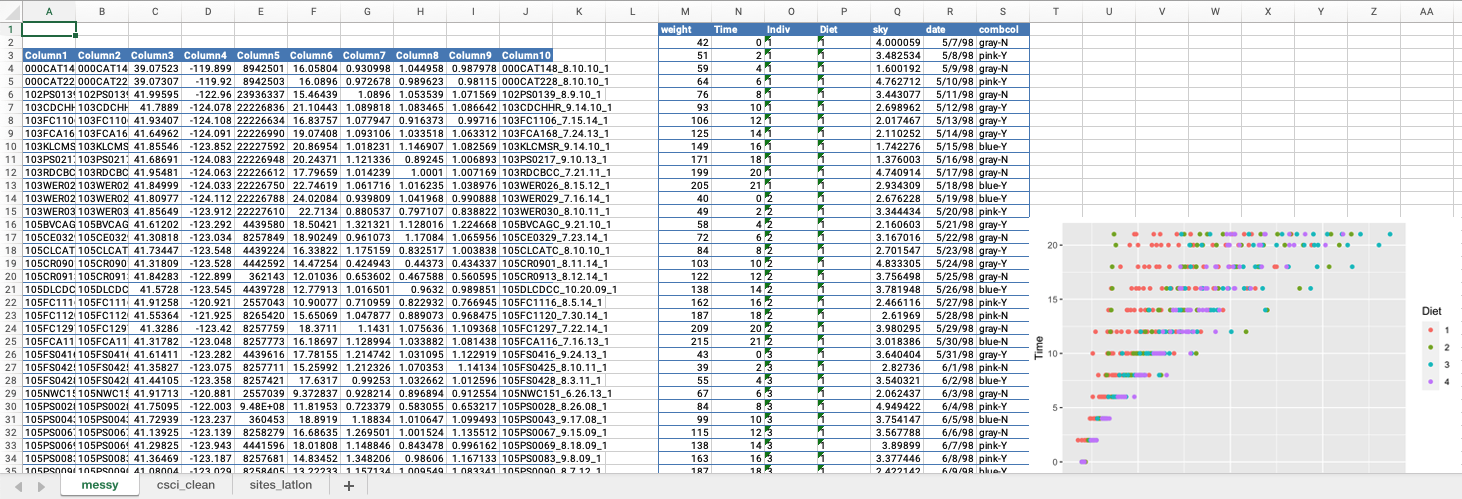
CHALLENGE 1
- What issues do you notice about the first tab?
- What could we do to make this tidy?
Click for Answers!
- Multiple tables on one sheet
- Figure embedded in the same sheet
- Tables start on different rows
- Table on far left doesn’t have column headers so no idea what the data may be
- Mixed data (see last column in middle table)
- Dates could be easily switched if order unknown
Extra Practice
Import Data from (Excel) Spreadsheets
Now that we have a general sense about what we may be up against, let’s take a look at how to get some data in a spreadsheet into R. For this we will need a few new packages! The R environment has many packages, and there may be others with similar capabilities, but let’s stick with these for now.
library(tidyverse)
library(openxlsx)
library(readxl)
Read data from a single tab
To start, let’s try to read in the first tab (the messy one) in our worksheet. The readxl::read_excel function is pretty straightforward for this, requiring us to know where the spreadsheet lives on our computer (our path), and the tab or sheet of interest. Arguments to the function are in yellow, and input values are in blue.
# load data
messy <- readxl::read_excel(path = "data/csci_spreadsheet.xlsx", sheet = 1)
Uh-oh. Something isn’t quite right here. Take a look at the interactive table below. Scroll to the right. What happened?
Ultimately the function read_excel did its job and read in our data. However, because our data table is not tidy, this would take a fair bit of extra wrangling to get the data into some sort of useable shape for analysis, plotting, etc.
So the take-home lesson here is that critically thinking about how data is entered and stored can save an immense amount of time in the long run, and it also makes it much easier to use a variety of tools when analyzing data.
Read in Some Tidy Data!
Ok, since we know that the data in tab 1 is a mess, let’s imagine that someone has cleaned this all up, and sent us a new version, with the tidy data in tabs 2 and 3. Let’s read these in!
CHALLENGE 2
- Read in sheet 2 (
csci_clean) and assign it to an object named “csci” - Read in sheet 3 (
sites_latlon) and assign it to an object named "sites
Click for Answers!
The only parts we need to change from the code above, are the sheet numbers, and the name of the objects.
csci <- readxl::read_excel(path = "data/csci_spreadsheet.xlsx", sheet = 2)
sites <- readxl::read_excel(path = "data/csci_spreadsheet.xlsx", sheet = 3)
Inspect & Wrangle the Data
It’s always a good idea to take a look at the data and make sure:
- we understand what all the pieces represent
- all the data is accounted for
- we know what sort of missing data or wrangling we may need to do
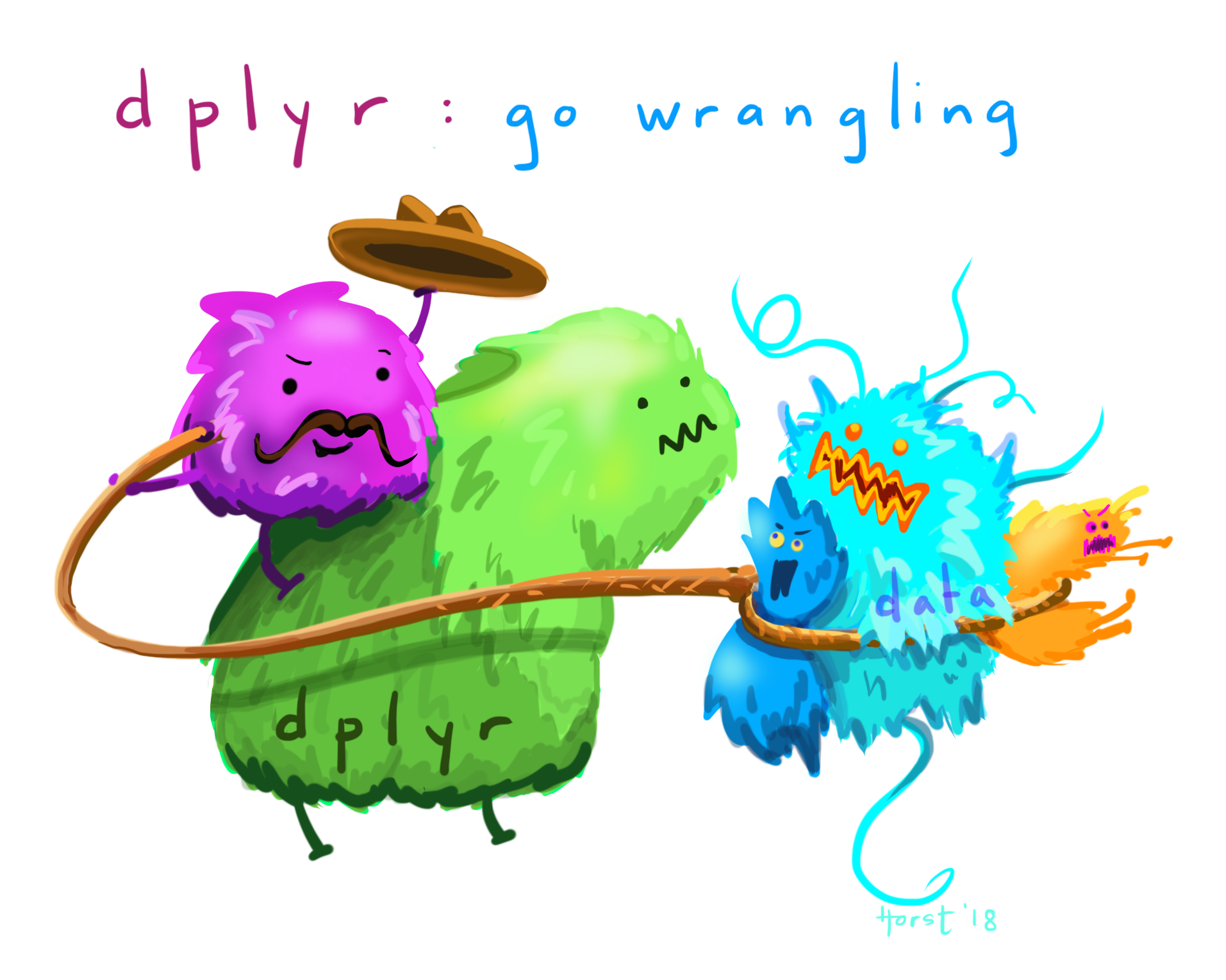
Figure 3: Artwork by @allison_horst
Inspect the sites Data
For our sites data, we have a set of bioassessment sites with StationID and latitude and longitude coordinates (awkwardly named New_Lat and New_Long). Here we can use glimpse() and head() as a way to look at the data types and columns present in the dataset.
glimpse(sites)## Rows: 1,613
## Columns: 3
## $ StationID <chr> "000CAT148", "000CAT228", "102PS0139", "103CDCHHR", "103FC1106", "103FCA168", "103KLCMSR", "103PS0217", "103RDCBCC", "103WER026", "103WER02…
## $ New_Lat <dbl> 39.07523, 39.07307, 41.99595, 41.78890, 41.93407, 41.64962, 41.85546, 41.68691, 41.95481, 41.84999, 41.80977, 41.85649, 41.61202, 41.30818,…
## $ New_Long <dbl> -119.8994, -119.9201, -122.9597, -124.0778, -124.1081, -124.0912, -123.8521, -124.0835, -124.0625, -124.0332, -124.1121, -123.9119, -123.29…head(sites)## # A tibble: 6 x 3
## StationID New_Lat New_Long
## <chr> <dbl> <dbl>
## 1 000CAT148 39.1 -120.
## 2 000CAT228 39.1 -120.
## 3 102PS0139 42.0 -123.
## 4 103CDCHHR 41.8 -124.
## 5 103FC1106 41.9 -124.
## 6 103FCA168 41.6 -124.Based on this, we know there are 1,613 rows (so 1,613 sites), and 3 columns. We know the StationID column is a character data class, and the other columns are numeric (or double which essentially means numbers with decimals).
Inspect the csci Data
The csci dataframe has the SampleID_old and _old.1 columns, the StationCode, and the bioassessment data for each sample (which contains a date). See [cite here] for more info on CSCI and the derivative metrics that it provides.
More Info on CSCI!
We can see the csci dataset is again, a mix of character and double data classes.
# structure (str) is similar to glimpse
str(csci)
## tibble [1,613 × 8] (S3: tbl_df/tbl/data.frame)
## $ SampleID_old : chr [1:1613] "000CAT148_8.10.10_1" "000CAT228_8.10.10_1" "102PS0139_8.9.10_1" "103CDCHHR_9.14.10_1" ...
## $ StationCode : chr [1:1613] "000CAT148" "000CAT228" "102PS0139" "103CDCHHR" ...
## $ COMID : num [1:1613] 8942501 8942503 23936337 22226836 22226634 ...
## $ E : num [1:1613] 16.1 16.1 15.5 21.1 16.8 ...
## $ OE : num [1:1613] 0.931 0.973 1.09 1.09 1.078 ...
## $ pMMI : num [1:1613] 1.045 0.99 1.054 1.083 0.916 ...
## $ CSCI : num [1:1613] 0.988 0.981 1.072 1.087 0.997 ...
## $ SampleID_old.1: chr [1:1613] "000CAT148_8.10.10_1" "000CAT228_8.10.10_1" "102PS0139_8.9.10_1" "103CDCHHR_9.14.10_1" ...Let’s use summary to look at the data a little differently.
# summary gives a quick assessment of numeric/date/factor data classes.
summary(csci[,c(3:7)])
## COMID E OE pMMI CSCI
## Min. : 342459 Min. : 3.677 Min. :0.0000 Min. :0.0126 Min. :0.1081
## 1st Qu.: 8272309 1st Qu.: 7.742 1st Qu.:0.6961 1st Qu.:0.5446 1st Qu.:0.6320
## Median : 17682470 Median :10.164 Median :0.9237 Median :0.7940 Median :0.8662
## Mean : 44272948 Mean :11.030 Mean :0.8732 Mean :0.7607 Mean :0.8172
## 3rd Qu.: 20364949 3rd Qu.:13.516 3rd Qu.:1.0733 3rd Qu.:0.9862 3rd Qu.:1.0182
## Max. :948090773 Max. :24.021 Max. :1.4164 Max. :1.4146 Max. :1.3797
## NA's :1 NA's :1Notice there are a few NA’s in there! We’ll keep those in mind as we move forward.
Tidy our Data
The typical steps for data analysis are usually something like:
- read the data in
- inspect the data
- tidy/wrangle the data
- save clean data
- make plots/do analysis
- report
- rinse and repeat
Using the same tools and process for each dataset can be immensely powerful.
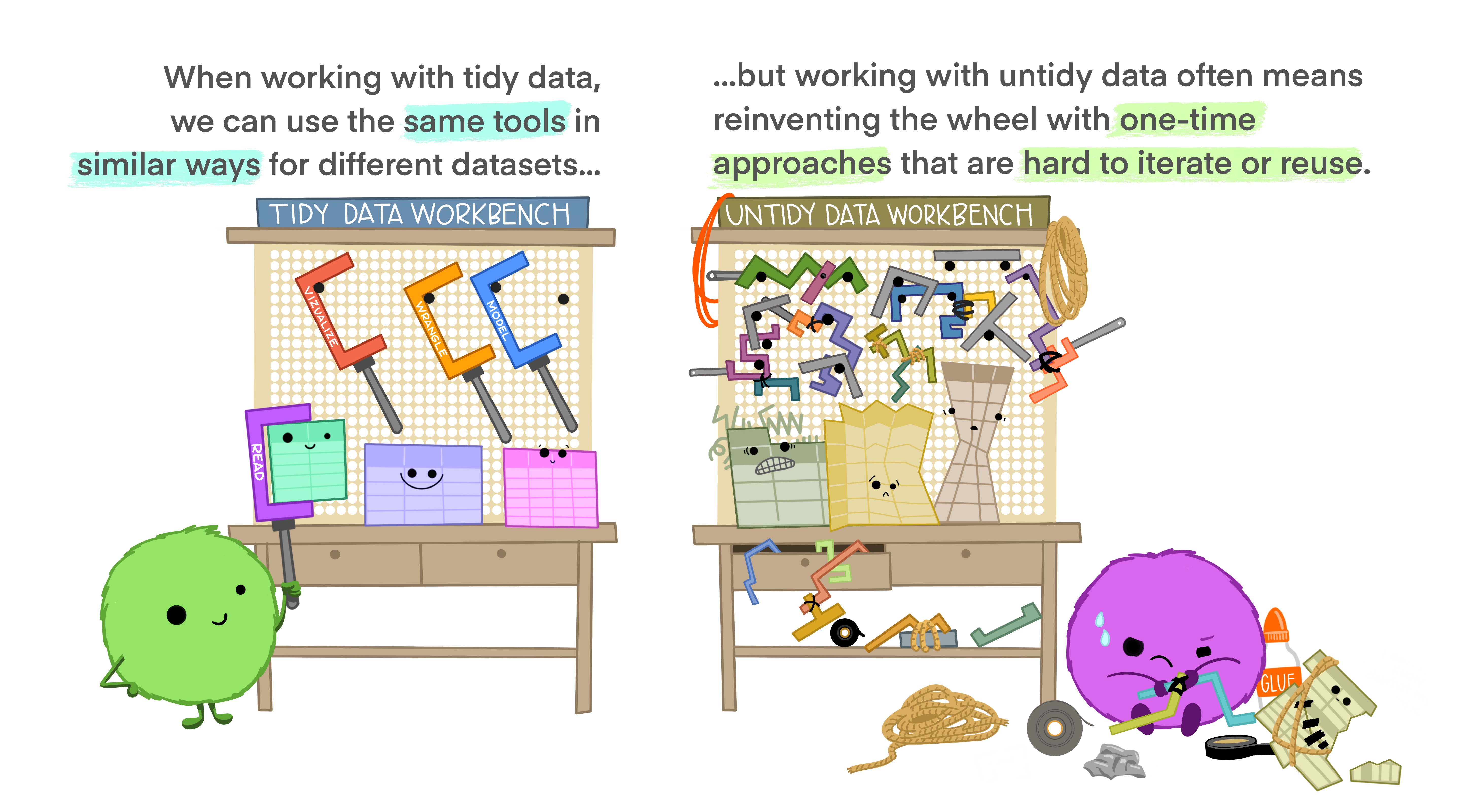
Figure 4: Illustrations from the Openscapes blog Tidy Data for reproducibility, efficiency, and collaboration by Julia Lowndes and Allison Horst
For now, we’ll keep this to a bare minimum, but sometimes the “cleaning & tidying” can require substantial time! Again, the cleaner and tidier the data in, the easier things will be.
Building on what we worked on in the first part of this workshop, let’s go ahead and use the dplyr package to do a few things, and then we’ll save our data out for the next steps.
First, let’s drop any NA’s from the csci data. Using a dplyr::filter is a great option.
csci_clean <- dplyr::filter(csci, !is.na(CSCI))

dim(csci_clean) # how many rows did we drop?
## [1] 1612 8Next, let’s rename a couple of the columns in the sites dataframe. Let’s simplify the New_Lat and New_Long columns.
sites_clean <- dplyr::rename(csci, lat = New_Lat, lon = New_Long)
# What happened?
Let’s try that again!
sites_clean <- dplyr::rename(sites, lat = New_Lat, lon = New_Long)
head(sites_clean)
## # A tibble: 6 x 3
## StationID lat lon
## <chr> <dbl> <dbl>
## 1 000CAT148 39.1 -120.
## 2 000CAT228 39.1 -120.
## 3 102PS0139 42.0 -123.
## 4 103CDCHHR 41.8 -124.
## 5 103FC1106 41.9 -124.
## 6 103FCA168 41.6 -124.Save it Out!
Let’s show how to save this back out as:
- a
csv - an RData file (
.RDataor.rda) - an RDS file (
.RDSor.rds) - a spreadsheet (
.xlsx)
The good thing is these mostly all involve the same basic code, with just a few minor tweaks.
Save to csv
Compared to a workbook, using csv is typically a better option. These files can be opened on any operating system, and they have a specific format which makes it harder to “untidy” things. Note, here we need to write two separate csv’s, one for each of our objects (csci_clean and sites_clean).
We can save to csv using either a tidyverse function write_csv, or the base R function write.csv. The main difference between the two, is the write_csv does not write row.names. Feel free to try both and open the file to see what’s different.
readr::write_csv(csci_clean, path="data/csci_clean.csv")## Warning: The `path` argument of `write_csv()` is deprecated as of readr 1.4.0.
## Please use the `file` argument instead.
## This warning is displayed once every 8 hours.
## Call `lifecycle::last_warnings()` to see where this warning was generated.readr::write_csv(sites_clean, path="data/sites_clean.csv")
# or try write.csv
# write.csv(csci_clean, file = "data/csci_cleaned.csv")
# we use read.csv() or read_csv() to read this back into RSave to .RData
RData files are a compressed R specific format, with some distinct advantages. For one, we can save multiple objects to a single .rda file. Another big benefit, is the data retains whatever format and structure that exists in your R environment…it will appear exactly as it was when you saved it. So, if you are going to be working in R exclusively, or working with folks who will be working in R, this can be a handy way to share data or analysis. These objects can be many things! One thing to note, whatever the object is named when it is saved will be what it is named when you reload this file back into R.
save(csci_clean, sites_clean, file = "data/csci_sites_clean.rda")

# we use load() to read this back into R
Save to .RDS
.RDS or .rds files are similar in type to .rda. They are R specific, they are compressed, but they are limited to a single object, and you can name this object whatever you choose when you re-import/read it back into R. Remember the difference between them by thinking of the S as “single” for a single object per .rds and the A as all objects (should you want to save everything into an .rda).
saveRDS(csci_clean, file="data/csci_clean.rds")
saveRDS(sites_clean, file="data/sites_clean.rds")
# we use readRDS() to read this back into R
Save to xlsx
Here we can use the openxlsx package to write our data. This is basically a 4-step process, first create a workbook, then create worksheets we can put our data in, then write the data to those worksheets, then save/write the whole workbook!
library(openxlsx)

wb <- createWorkbook() # first create the workbook

# then create the worksheets we want to write data to
addWorksheet(wb, sheetName = "csci_clean", gridLines = TRUE)
addWorksheet(wb, sheetName = "sites_clean", gridLines = TRUE)

# now we add our cleaned data
writeDataTable(wb=wb, sheet=1, x = csci_clean, withFilter = FALSE)
writeDataTable(wb=wb, sheet=2, x = sites_clean, withFilter = FALSE)

# now we save our data
saveWorkbook(wb, "data/csci_sites_clean_spreadsheet.xlsx", overwrite = TRUE)
Great work! Let’s move to the next lesson.