Wrangling Data
Objectives for this section:
- learn how to tidy and manipulate datasets
- use the pipe (
%>%) to combine operations
Data wrangling with {dplyr}
Data wrangling is the part of any data analysis that will take the most time. While it may not necessarily be fun, it is foundational to all the work that follows. Often, it also takes significantly longer than actually performing the data analysis or creating a data visualization, so do not panic if, in the future, you find yourself spending a lot of time on this single step. For the purpose of condensing today’s lessons, we will be working with a fairly tidy dataset. But there are many online resources available to help you in your own work, should you be handed a project with a particularly gnarly dataset.

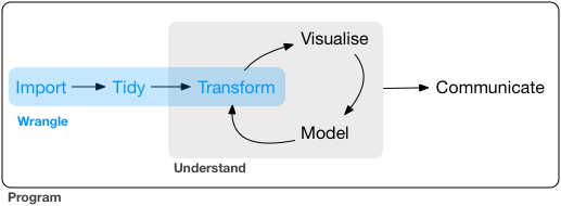
Figure 1: Image from “R for Data Science” by Garrett Grolemund and Hadley Wickham.
The data wrangling process includes data import, tidying, and transformation. The process directly feeds into, and is not mutually exclusive with, the understanding or modeling side of data exploration. More generally, data wrangling is the manipulation or combination of datasets for the purpose of analysis.
All wrangling is based on a purpose. No one wrangles for the sake of wrangling (usually), so the process always begins by answering the following two questions:
- What do my input data look like?
- What should my data look like given what I want to do?
At the most basic level, going from what your data looks like to what it should look like will require a few key operations. Some common examples:
- Selecting specific variables
- Filtering observations by some criteria
- Adding or modifying existing variables
- Renaming variables
- Arranging rows by a variable
- Summarizing a variable conditional on others
The {dplyr} package provides easy tools for these common data manipulation tasks and is a core package from the {tidyverse} suite of packages. The philosophy of {dplyr} is that one function does one thing and the name of the function says what it does.
We’ll start this lesson by working in the script we created in the previous section: cabw_script_day1.R.
Below your code that imports the dataset, let’s make a new section! Go to Code > Insert Section, and type your new section header Wrangling and Plotting. We can also use keyboard shortcuts for this (Ctrl or ⌘ + Shift + R). You should notice how this now appears in an expandable table of contents on the right hand side of your script pane (look for the tiny button that has little gray horizontal lines on it). This feature can be very helpful in keep your scripts organized.
Alright, let’s get wrangling!
(Re)-Load Our Data
Any reproducible analysis should be able to start from scratch, and rebuild all the parts, sometimes over and over again. For that reason, it’s a good habit to get into to Restart your R Session. Sometimes this solves issues, sometimes it’s just good to make sure everything runs up to the point you are working. Let’s do that now!
- Go to
Session>Restart R! - Check your
Environmenttab…it should be empty! - Now we need to re-load our library, and re-load our data.
Challenge 1
Load {tidyverse} package into R.
Load or read the
csciandascidatasets into R. Comment your code!Save your script.
Click for Answers!
# load the library
library(tidyverse)

# Load CSCI and ASCI datasets.
cscidat <- read_csv('data/cscidat.csv')
ascidat <- read_csv('data/ascidat.csv')

# check environment, both are there!
Selecting
Our goal with the datasets we have loaded in is to combine the bioassessment scores by each unique location, date, and replicate, while keeping only the data we need for our plots.
The select function lets you retain or exclude columns.
# first, select some chosen columns
dplyr_sel1 <- select(cscidat, SampleID_old, New_Lat, New_Long, CSCI)

# examine those columns
head(dplyr_sel1)
## # A tibble: 6 x 4
## SampleID_old New_Lat New_Long CSCI
## <chr> <dbl> <dbl> <dbl>
## 1 000CAT148_8.10.10_1 39.1 -120. 0.988
## 2 000CAT228_8.10.10_1 39.1 -120. 0.981
## 3 102PS0139_8.9.10_1 42.0 -123. 1.07
## 4 103CDCHHR_9.14.10_1 41.8 -124. 1.09
## 5 103FC1106_7.15.14_1 41.9 -124. 0.997
## 6 103FCA168_7.24.13_1 41.6 -124. 1.06# select everything but CSCI and COMID: the "-" sign indicates "not"
dplyr_sel2 <- select(cscidat, -CSCI, -COMID)
head(dplyr_sel2)## # A tibble: 6 x 8
## SampleID_old StationCode New_Lat New_Long E OE pMMI SampleID_old.1
## <chr> <chr> <dbl> <dbl> <dbl> <dbl> <dbl> <chr>
## 1 000CAT148_8.10.10_1 000CAT148 39.1 -120. 16.1 0.931 1.04 000CAT148_8.10.10_1
## 2 000CAT228_8.10.10_1 000CAT228 39.1 -120. 16.1 0.973 0.990 000CAT228_8.10.10_1
## 3 102PS0139_8.9.10_1 102PS0139 42.0 -123. 15.5 1.09 1.05 102PS0139_8.9.10_1
## 4 103CDCHHR_9.14.10_1 103CDCHHR 41.8 -124. 21.1 1.09 1.08 103CDCHHR_9.14.10_1
## 5 103FC1106_7.15.14_1 103FC1106 41.9 -124. 16.8 1.08 0.916 103FC1106_7.15.14_1
## 6 103FCA168_7.24.13_1 103FCA168 41.6 -124. 19.1 1.09 1.03 103FCA168_7.24.13_1# select columns that contain the letter c
dplyr_sel3 <- select(cscidat, matches('c'))
head(dplyr_sel3)## # A tibble: 6 x 3
## StationCode COMID CSCI
## <chr> <dbl> <dbl>
## 1 000CAT148 8942501 0.988
## 2 000CAT228 8942503 0.981
## 3 102PS0139 23936337 1.07
## 4 103CDCHHR 22226836 1.09
## 5 103FC1106 22226634 0.997
## 6 103FCA168 22226990 1.06# Note, these datasets should all be appearing in your Environment pane in the upper right hand corner of your screen as you continue.Filtering
After selecting columns, you’ll probably want to remove observations that don’t fit some criteria. For example, maybe you want to remove CSCI scores less than some threshold, find stations above a certain latitude, or both.
# get CSCI scores greater than 0.79
dplyr_filt1 <- filter(cscidat, CSCI > 0.79)
head(dplyr_filt1)
## # A tibble: 6 x 10
## SampleID_old StationCode New_Lat New_Long COMID E OE pMMI CSCI SampleID_old.1
## <chr> <chr> <dbl> <dbl> <dbl> <dbl> <dbl> <dbl> <dbl> <chr>
## 1 000CAT148_8.10.10_1 000CAT148 39.1 -120. 8942501 16.1 0.931 1.04 0.988 000CAT148_8.10.10_1
## 2 000CAT228_8.10.10_1 000CAT228 39.1 -120. 8942503 16.1 0.973 0.990 0.981 000CAT228_8.10.10_1
## 3 102PS0139_8.9.10_1 102PS0139 42.0 -123. 23936337 15.5 1.09 1.05 1.07 102PS0139_8.9.10_1
## 4 103CDCHHR_9.14.10_1 103CDCHHR 41.8 -124. 22226836 21.1 1.09 1.08 1.09 103CDCHHR_9.14.10_1
## 5 103FC1106_7.15.14_1 103FC1106 41.9 -124. 22226634 16.8 1.08 0.916 0.997 103FC1106_7.15.14_1
## 6 103FCA168_7.24.13_1 103FCA168 41.6 -124. 22226990 19.1 1.09 1.03 1.06 103FCA168_7.24.13_1# get CSCI scores above latitude 37N
dplyr_filt2 <- filter(cscidat, New_Lat > 37)
head(dplyr_filt2)## # A tibble: 6 x 10
## SampleID_old StationCode New_Lat New_Long COMID E OE pMMI CSCI SampleID_old.1
## <chr> <chr> <dbl> <dbl> <dbl> <dbl> <dbl> <dbl> <dbl> <chr>
## 1 000CAT148_8.10.10_1 000CAT148 39.1 -120. 8942501 16.1 0.931 1.04 0.988 000CAT148_8.10.10_1
## 2 000CAT228_8.10.10_1 000CAT228 39.1 -120. 8942503 16.1 0.973 0.990 0.981 000CAT228_8.10.10_1
## 3 102PS0139_8.9.10_1 102PS0139 42.0 -123. 23936337 15.5 1.09 1.05 1.07 102PS0139_8.9.10_1
## 4 103CDCHHR_9.14.10_1 103CDCHHR 41.8 -124. 22226836 21.1 1.09 1.08 1.09 103CDCHHR_9.14.10_1
## 5 103FC1106_7.15.14_1 103FC1106 41.9 -124. 22226634 16.8 1.08 0.916 0.997 103FC1106_7.15.14_1
## 6 103FCA168_7.24.13_1 103FCA168 41.6 -124. 22226990 19.1 1.09 1.03 1.06 103FCA168_7.24.13_1# use both filters
dplyr_filt3 <- filter(cscidat, CSCI > 0.79 & New_Lat > 37)
head(dplyr_filt3)## # A tibble: 6 x 10
## SampleID_old StationCode New_Lat New_Long COMID E OE pMMI CSCI SampleID_old.1
## <chr> <chr> <dbl> <dbl> <dbl> <dbl> <dbl> <dbl> <dbl> <chr>
## 1 000CAT148_8.10.10_1 000CAT148 39.1 -120. 8942501 16.1 0.931 1.04 0.988 000CAT148_8.10.10_1
## 2 000CAT228_8.10.10_1 000CAT228 39.1 -120. 8942503 16.1 0.973 0.990 0.981 000CAT228_8.10.10_1
## 3 102PS0139_8.9.10_1 102PS0139 42.0 -123. 23936337 15.5 1.09 1.05 1.07 102PS0139_8.9.10_1
## 4 103CDCHHR_9.14.10_1 103CDCHHR 41.8 -124. 22226836 21.1 1.09 1.08 1.09 103CDCHHR_9.14.10_1
## 5 103FC1106_7.15.14_1 103FC1106 41.9 -124. 22226634 16.8 1.08 0.916 0.997 103FC1106_7.15.14_1
## 6 103FCA168_7.24.13_1 103FCA168 41.6 -124. 22226990 19.1 1.09 1.03 1.06 103FCA168_7.24.13_1# You can use "&" to signify "and" and "|" to signify "or" in your wrangling statements.
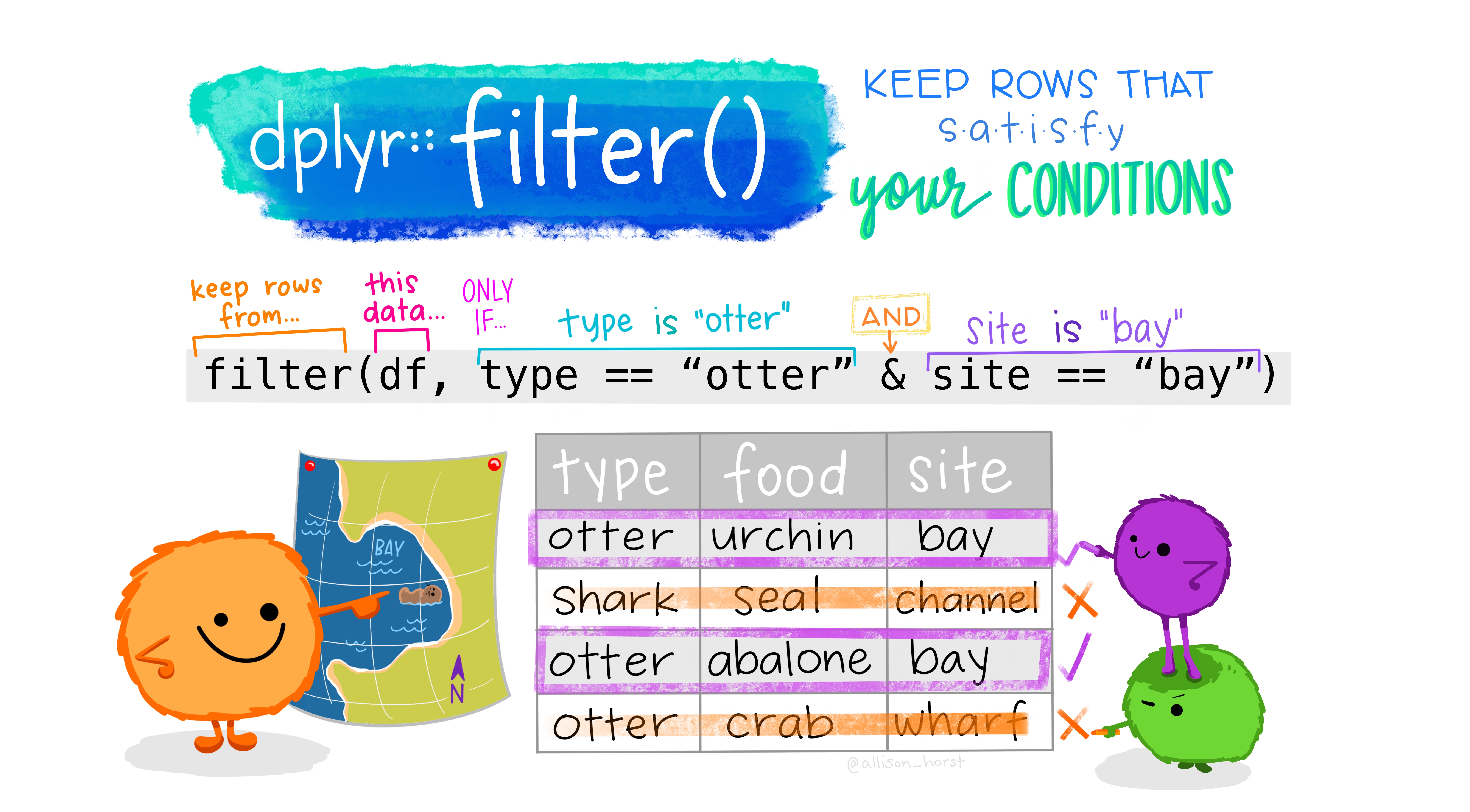
Figure 2: Illustration by @allison_horst.
Filtering can take a bit of time to master because there are several ways to tell R what you want. To use filtering effectively, you have to know how to select the observations that you want using the comparison operators. R provides the standard suite: >, >=, <, <=, != (not equal), and == (equal). Remember to use = instead of == when testing for equality!
Mutating
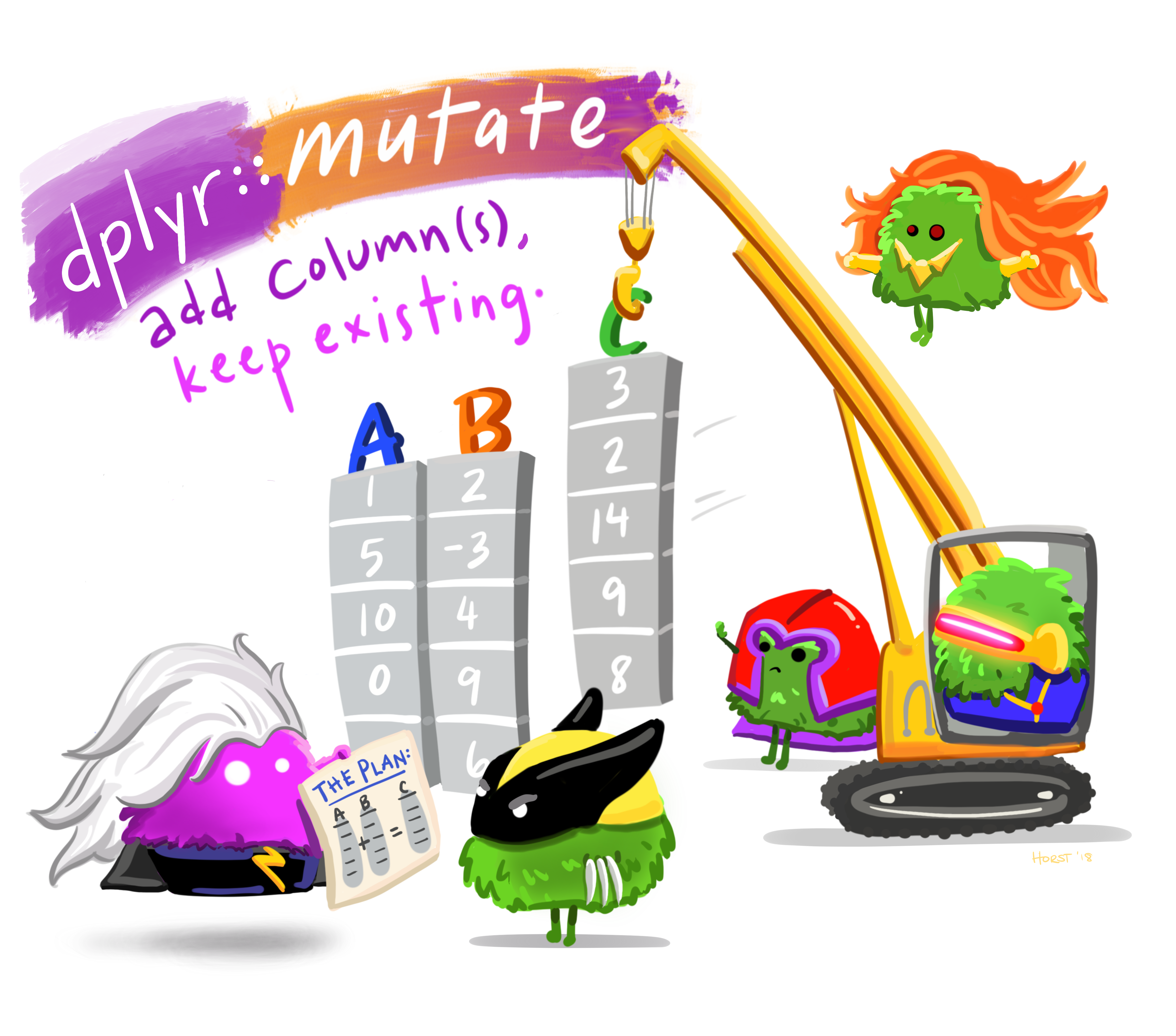
Now that we’ve seen how to select columns and filter observations of a data frame, maybe we want to add a new column. In dplyr, mutate allows us to add new columns. These can be vectors you are adding or based on expressions applied to existing columns. For instance, maybe we want to convert a numeric column into a categorical using certain criteria or maybe we want to make a new column based on some arithmetic on other columns.
# get observed taxa
dplyr_mut1 <- mutate(cscidat, observed = OE * E)
head(dplyr_mut1)
## # A tibble: 6 x 11
## SampleID_old StationCode New_Lat New_Long COMID E OE pMMI CSCI SampleID_old.1 observed
## <chr> <chr> <dbl> <dbl> <dbl> <dbl> <dbl> <dbl> <dbl> <chr> <dbl>
## 1 000CAT148_8.10.10_1 000CAT148 39.1 -120. 8942501 16.1 0.931 1.04 0.988 000CAT148_8.10.10_1 14.9
## 2 000CAT228_8.10.10_1 000CAT228 39.1 -120. 8942503 16.1 0.973 0.990 0.981 000CAT228_8.10.10_1 15.7
## 3 102PS0139_8.9.10_1 102PS0139 42.0 -123. 23936337 15.5 1.09 1.05 1.07 102PS0139_8.9.10_1 16.9
## 4 103CDCHHR_9.14.10_1 103CDCHHR 41.8 -124. 22226836 21.1 1.09 1.08 1.09 103CDCHHR_9.14.10_1 23.
## 5 103FC1106_7.15.14_1 103FC1106 41.9 -124. 22226634 16.8 1.08 0.916 0.997 103FC1106_7.15.14_1 18.1
## 6 103FCA168_7.24.13_1 103FCA168 41.6 -124. 22226990 19.1 1.09 1.03 1.06 103FCA168_7.24.13_1 20.9# add a column for lo/hi csci scores
dplyr_mut2 <- mutate(cscidat, CSCIcat = ifelse(CSCI <= 0.79, 'lo', 'hi'))
head(dplyr_mut2)## # A tibble: 6 x 11
## SampleID_old StationCode New_Lat New_Long COMID E OE pMMI CSCI SampleID_old.1 CSCIcat
## <chr> <chr> <dbl> <dbl> <dbl> <dbl> <dbl> <dbl> <dbl> <chr> <chr>
## 1 000CAT148_8.10.10_1 000CAT148 39.1 -120. 8942501 16.1 0.931 1.04 0.988 000CAT148_8.10.10_1 hi
## 2 000CAT228_8.10.10_1 000CAT228 39.1 -120. 8942503 16.1 0.973 0.990 0.981 000CAT228_8.10.10_1 hi
## 3 102PS0139_8.9.10_1 102PS0139 42.0 -123. 23936337 15.5 1.09 1.05 1.07 102PS0139_8.9.10_1 hi
## 4 103CDCHHR_9.14.10_1 103CDCHHR 41.8 -124. 22226836 21.1 1.09 1.08 1.09 103CDCHHR_9.14.10_1 hi
## 5 103FC1106_7.15.14_1 103FC1106 41.9 -124. 22226634 16.8 1.08 0.916 0.997 103FC1106_7.15.14_1 hi
## 6 103FCA168_7.24.13_1 103FCA168 41.6 -124. 22226990 19.1 1.09 1.03 1.06 103FCA168_7.24.13_1 hi# Note: "ifelse" statements can be very helpful for conditional assignments. Their basic structure is if *the criteria* is met, then print 'this', if not, then print 'that'.
# So, the actual statement may look something like:
# ifelse(*the criteria*, 'this', 'that')
Figure 3: Illustration by @allison_horst.
More functions
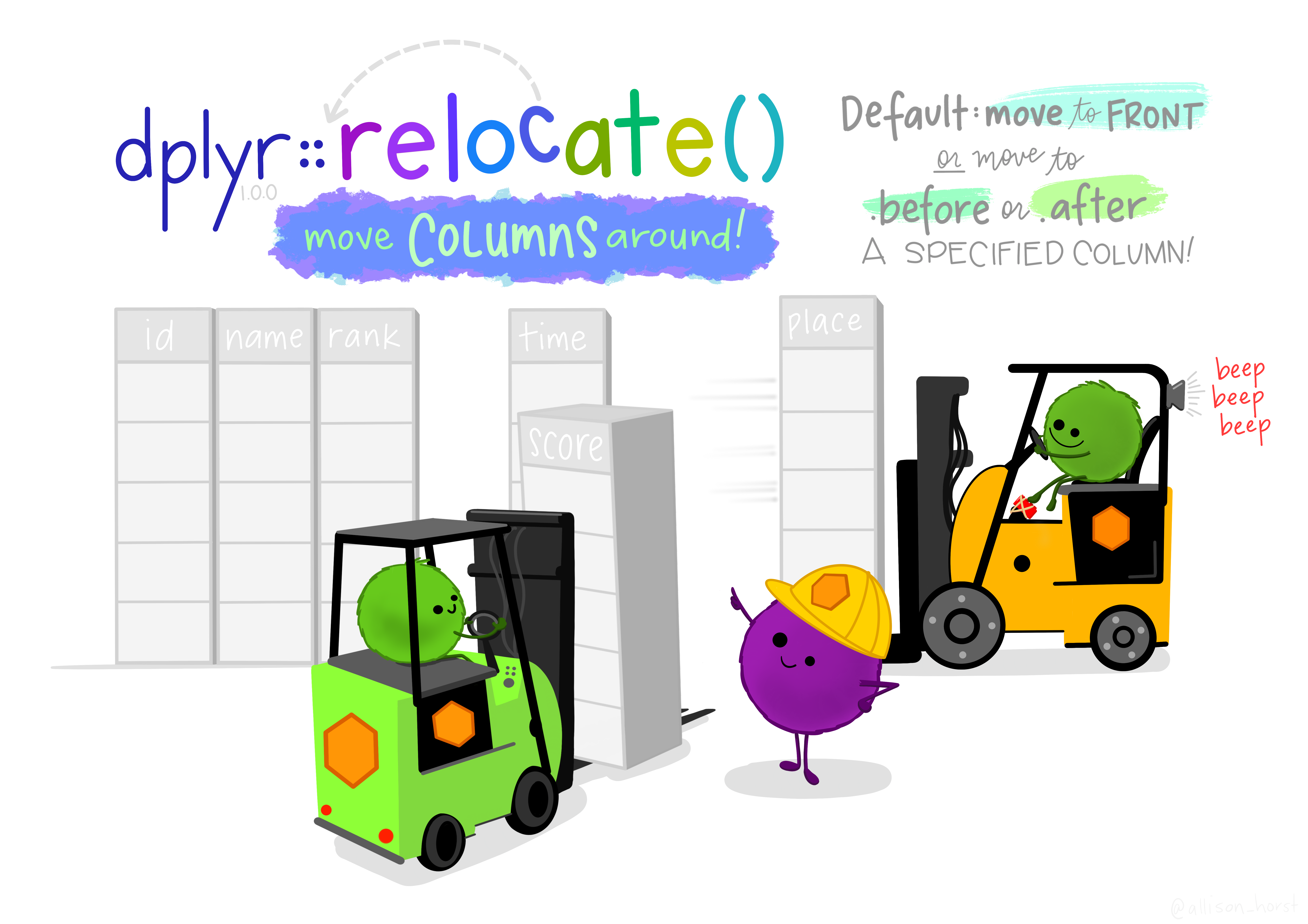
Some other useful dplyr functions include arrange to sort the observations (rows) by a column and rename to (you guessed it) rename a column.
# arrange by CSCI scores
dplyr_arr <- arrange(cscidat, CSCI)
head(dplyr_arr)
## # A tibble: 6 x 10
## SampleID_old StationCode New_Lat New_Long COMID E OE pMMI CSCI SampleID_old.1
## <chr> <chr> <dbl> <dbl> <dbl> <dbl> <dbl> <dbl> <dbl> <chr>
## 1 206PS0073_7.20.10_1 206PS0073 38.1 -123. 1669863 13.3 0.150 0.0663 0.108 206PS0073_7.20.10_1
## 2 205R01390_5.23.13_1 205R01390 37.5 -122. 17692585 13.1 0.152 0.0852 0.119 205R01390_5.23.13_1
## 3 205R00878_4.24.13_1 205R00878 37.6 -122. 17691075 14.0 0.214 0.0336 0.124 205R00878_4.24.13_1
## 4 801S03971_6.16.14_1 801S03971 33.7 -118. 20355412 8.23 0.0729 0.231 0.152 801S03971_6.16.14_1
## 5 204R00383_6.11.12_1 204R00383 37.7 -122. 2804015 10.7 0.281 0.0325 0.157 204R00383_6.11.12_1
## 6 204R00583_6.13.12_1 204R00583 37.6 -122. 2804187 13.3 0.278 0.0448 0.162 204R00583_6.13.12_1# rename lat/lon (note the format of newName = oldName)
dplyr_rnm <- rename(cscidat,
lat = New_Lat,
lon = New_Long
)
head(dplyr_rnm)## # A tibble: 6 x 10
## SampleID_old StationCode lat lon COMID E OE pMMI CSCI SampleID_old.1
## <chr> <chr> <dbl> <dbl> <dbl> <dbl> <dbl> <dbl> <dbl> <chr>
## 1 000CAT148_8.10.10_1 000CAT148 39.1 -120. 8942501 16.1 0.931 1.04 0.988 000CAT148_8.10.10_1
## 2 000CAT228_8.10.10_1 000CAT228 39.1 -120. 8942503 16.1 0.973 0.990 0.981 000CAT228_8.10.10_1
## 3 102PS0139_8.9.10_1 102PS0139 42.0 -123. 23936337 15.5 1.09 1.05 1.07 102PS0139_8.9.10_1
## 4 103CDCHHR_9.14.10_1 103CDCHHR 41.8 -124. 22226836 21.1 1.09 1.08 1.09 103CDCHHR_9.14.10_1
## 5 103FC1106_7.15.14_1 103FC1106 41.9 -124. 22226634 16.8 1.08 0.916 0.997 103FC1106_7.15.14_1
## 6 103FCA168_7.24.13_1 103FCA168 41.6 -124. 22226990 19.1 1.09 1.03 1.06 103FCA168_7.24.13_1Some More Practice?
Let’s take a look at some practice challenges to work on the various functions we’ve described above. Let’s clean up our CSCI dataset in preparation to join with our ASCI dataset. We’ll select columns we want and rename columns with odd names to create a more tidy dataset.
Challenge 2
- Select the unique sample ID column (
SampleID_old), latitude (New_Lat), longitude (New_Long), andCSCIcolumns. Reassign these columns to a new dataset namedcscidat_trim, so we don’t overwrite the existing dataset.
Click for Answers!
cscidat_trim <- select(cscidat, SampleID_old, New_Lat, New_Long, CSCI)Challenge 3
- Rename the
SampleID_oldcolumn toid,New_Lattolat, andNew_Longtolon.
Click for Answers!
cscidat_trim <- rename(cscidat,
                       id = SampleID_old,
                       lat = New_Lat,
                       lon = New_Long
)
Piping using the tidyverse
Each of the functions we learned above - select(), filter(), mutate(), and more - can be used on their own. However, a particularly powerful application of the {tidyverse} package is the ability to “pipe” or perform multiple functions all in one go.
In order to do so, you must use the symbols %>%, otherwise known as a pipe. When placed between functions in your code, this allows you to perform multiple operations on a single dataset.
Typically, piping will assume the following format:
<NEW DATASET> <- <OLD DATASET> %>%
  <FIRST_FUNCTION> %>%
  <SECOND_FUNCTION> %>%
  <THIRD_FUNCTION> %>%
    etc.
So, if you wanted to perform many of the operations we practiced above, we could use %>% to create a new dataset (csci_new) by typing the following:
csci_new <- cscidat %>% # Use the original dataset and then...
    select(CSCI, COMID, New_Lat) %>% # select only CSCI, COMID, and latitude columns and then...
    filter(New_Lat > 37) %>% # filter for Latitudes above 37 and then...
    mutate(CSCIcat = ifelse(CSCI <= 0.79, 'lo', 'hi')) # new column with categories according to CSCI.
More Practice!
Let’s practice piping just a bit more before we move onto plotting our data.
Challenge 4
- Using the piping technique and the
ascidatdataset, create a new dataset calledasci_newthat includes:
- Site type and ASCI
- Only sites identified as “Reference”
- A new column with ASCI scores multiplied by 10
Check the dimensions of the new dataset (Hint: Use the
View()function).Save your script!
Click for Answers!
asci_new <- ascidat %>% # Use the original dataset and then...
  select(ASCI, site_type) %>% # select only ASCI and site type columns and then...
  filter(site_type == "Reference") %>% # filter for reference sites only and then...
  mutate(ASCI_10 = ASCI*10) # new column with ASCI values multiplied by 10.

dim(asci_new)
## [1] 737 3This concludes the “wrangling data” section of our R workshop today. If you are experiencing any problems or have a question, please send Ryan, Heili, or one of the workshop assistants a message in the chat.
If you would like to learn more about the possibilities withing the dplyr package, here are some additional resources:

Figure 4: Illustration by @allison_horst.
Great work! Let’s move to the next lesson.