Importing Data
Objectives for this section:
- get organized at the start of each new project
- create and save an .R script
- import data from a
.csv
Getting organized
Today, as you learn new concepts and utilities in R, we will also be teaching you how to set up your workflow so that you and your collaborators can use R more efficiently. By taking the time at the very beginning of a project to maintain code that is well organized and clear, you will create analyses that are more reproducible and shareable. And, when you come back to your files years later, you can pick back up right where you left off.
Before you start working on a new dataset in RStudio, it is very important that you create a place to store your files. Starting off organized and staying organized in R will make future you so much happier. So, we’re going to encourage that you take a moment now to organize your files and keep things tidy.
RStudio projects
I strongly encourage you to use RStudio projects when you are working with R. The RStudio project provides a central location for working on a particular task. It helps with file management and is portable because all the files live in the same project. RStudio projects also remember history - what commands you used and what data objects are in your Environment.
To create a new project, click on the File menu at the top of the RStudio window and select New project...
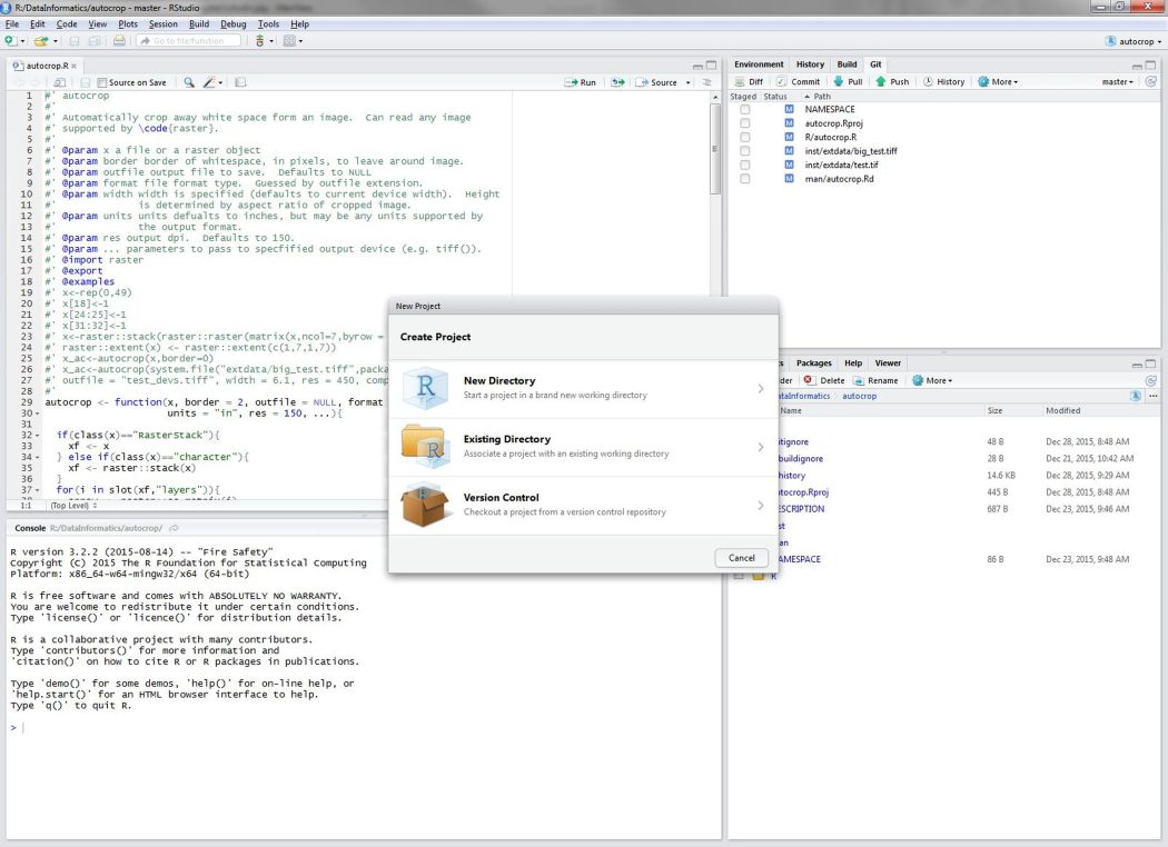
Figure 1: Beginning a new project in RStudio.
Select New Directory > New Project. Title this project “cabw_r_workshop” (we will use this directory for the rest of today’s workshop), and save it on your computer in a place that is logical and easy for you to find in the future. Then, click “Create Project.” In the RStudio window that just opened, you should now see your working directory printed along the top of the screen (e.g., ~/Desktop/cabw_r_workshop).
Now, we can use this project for our data and any scripts we create.
Scripting
Up until this point, we have been working in the Console. In most cases, you will not enter and execute code directly in the Console but rather type and edit code in a script and then send it to the Console when you’re ready to run it. The key difference here is that a script can be saved and shared.
To open a new script, navigate to the File menu, and select New File > R Script:
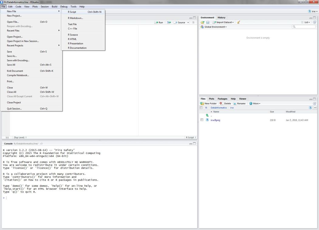
Figure 2: Opening a new script in RStudio.
Save that file into your newly created project and name it cabw_script_day1.R. It’ll just be a blank text file at this point.
A script works similarly to the Console, but it does have a few key differences. The first, is that you can add text that is not able to be run. This text is referred to as annotations or comments, and it is denoted by using a pound symbol or hashtag (#) prior to the text. Let’s use this to add a title, name, and date to our new script.
# CABW 2020 Bioassessment R Tutorial
# Firstname Lastname
# October 13, 2020
Let’s practice making variables in our script or .R file. Type the following into your script:
#### Variables ####

# Create a new variable.
fish <- 10 + 45
After you write your script it can be sent to the Console to run the code in R. Any variables you create in your script will not be available in your working environment until this is done. There are two ways to send code to the console. First, you can hit the Run button at the top right of the scripting window. Second, and preferred, you can use Ctrl+enter or ⌘+Enter on a Mac. Both approaches will send the selected line to the console, then move to the next line in your script. You can also highlight and send an entire block of code. If you’d like to run all the code in your script at once, you can use Ctrl or ⌘+shift +enter.
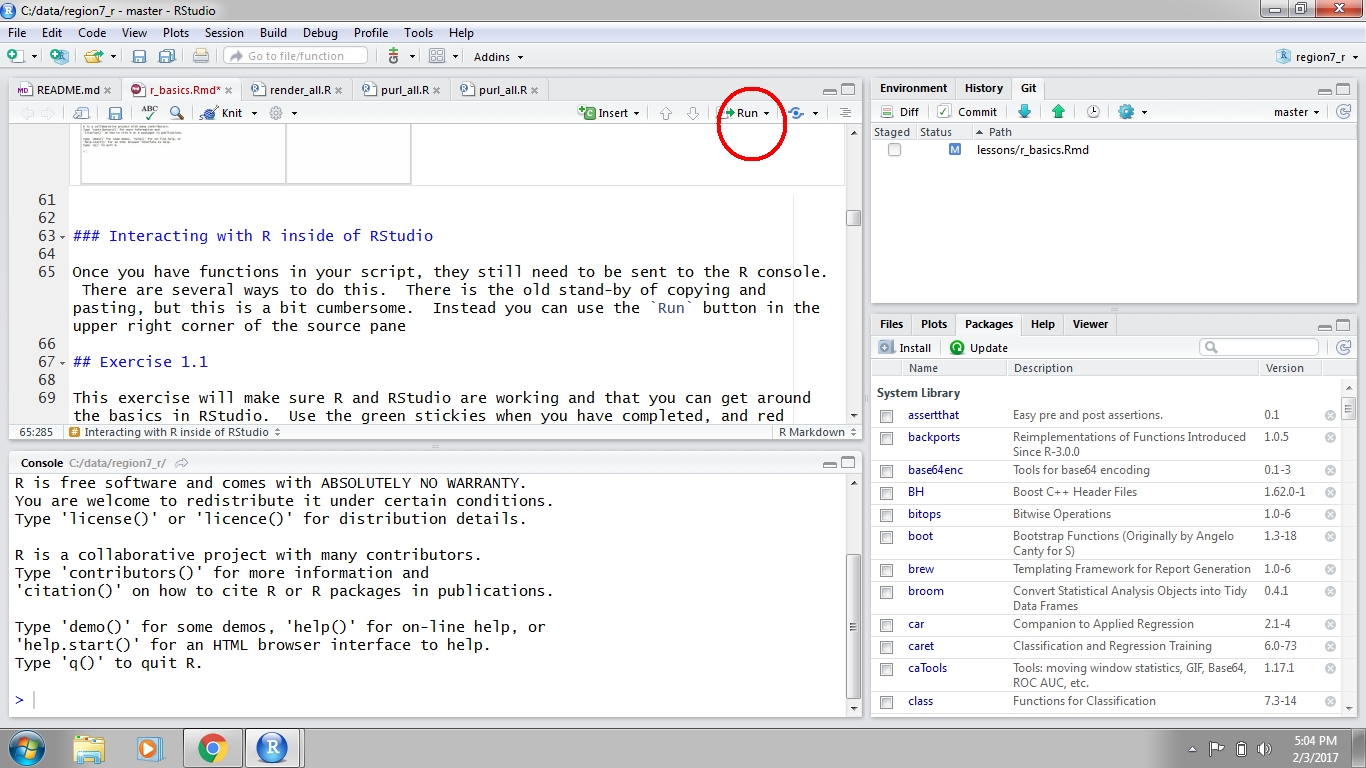
Figure 3: Running code in RStudio.
Place your cursor on the line where you’ve created the fish variable, and run the line of code. Check to be certain that this variable has now appeared in your Environment.
Add the following lines of code to your script, and then run each one:
# Create additional variables.
nitrogen <- 79 - 15
algae <- fish * nitrogen
For the remainder of the workshop, we’ll use this script (cabw_script_day1.R) instead of the Console. For comparison, working in the Console is like sending a lot of text messages, but working in this new script file is more like working in Word–you can save, edit, and track your changes, not to mention more easily collaborate with others to write files.
PRACTICE
Create variables named
riffleandpoolin your script, and assign a number to each.Annotate your variables with a comment using the
#notation so future you (or colleagues and collaborators) understands what you’ve done.Run each of your new variables to be sure they appear in your
Environment.Save your script.
Click for Answers!
# Let's make a variable named riffle and assign a number to it
riffle <- 100

# let's make a variable named pool and assign a list of numbers
# to make a list of anything, we use "c( )" for "concatenate" or "combine"
pool <- c(10, 20, 30)

# And we can save with Cmd + S or Ctrl + S, or File > Save!
If you have any difficulty completing the above 4 steps, please send a message to Ryan, Heili, or one of the workshop assistants in the chat.
We have demonstrated that scripts are just as powerful as the Console, and they are much more useful, because they can be re-used, shared, and re-run, making any analysis reproducible. Think of all the mouse clicks it may take to make or do something, and imagine instead using **Run** once on a script to recreate an entire history of those clicks. So, let’s continue working in the script by loading packages and datasets we’ll use for this workshop.
Installing packages
At the beginning of most of your scripts, you will need to tell R which packages or libraries (lots of pieces of code we can use for specific tasks) it needs to use to run the code below. So, we’re going to install and load some additional packages for this week’s workshop.
In the Console, type and run the following lines of code:
install.packages("sf")
install.packages("mapview")
install.packages("viridis")
install.packages("USAboundaries")
We run these installations in the Console, because they only need to happen once per person, and once installed, R will recognize them in perpetuity.
Loading Libraries
An important note, a package is a library of functions (which are code that we can use to do specific tasks with). Packages usually have a theme or a group of functions that are oriented around a similar topic. Some may just be a bunch of functions that are all useful in different ways, like a utility belt. Either way, we install a package once per R version, and we load our library once per R session (so each time we want to work in a script in R).
Let’s add the following to our script file and run each line to attach our libraries of functions for use today. For now, we will just be using the {tidyverse} package.
# Load packages into R so they are accessible for our session:
library("tidyverse")
Getting your data into R
It is the rare case when you manually enter your data in R, not to mention impractical for most datasets. Most data analysis workflows typically begin with importing a dataset from an external source. This means committing a dataset to memory (i.e., storing it as a variable) as one of R’s data structure formats.
You should have downloaded today’s dataset already, but if not, the data are available here. The data are in a zipped folder. Download the file to your computer (anywhere).
Create a new folder in your cabw_r_workshop project named data and move the datazip.zip file into this location. You will need to unzip this folder with whatever option you have for your system (Unzip, 7Zip, etc). Now, you should see them appear in the Files tab under the data folder in the lower right hand corner of your RStudio window - this means the files are now a part of the same working directory as your script.
Flat data files (text only, rectangular format) present the least complications on import because there is very little to assume about the structure of the data. On import, R tries to guess the data type for each column, and this is fairly unambiguous with flat files.The base installation of R comes with some easy to use functions for importing flat files, but we’re going to use the read_csv() function from the readr package, which you’ve already loaded in through the {tidyverse}. R comes with a built in function read.csv(), but we’re going to use read_csv() because it handles a few defaults more cleanly, and can be slightly faster reading in data.
Now that we have the data downloaded and extracted to our data folder, we’ll use read_csv() to import two files.
Type the following in your script. Note the use of relative file paths within your project.
# Load CSCI and ASCI datasets.
cscidat <- read_csv('data/cscidat.csv')
ascidat <- read_csv('data/ascidat.csv')
Send the commands to the console with Ctrl or ⌘+Enter.
Verify that the data imported correctly by viewing the datasets in a spreadsheet style in a new window:
# examine datasets in new windows
View(cscidat)
View(ascidat)
Inspect the Data
Let’s explore the datasets a bit. There are many useful functions for exploring the characteristics of a dataset. This is always a good idea when you first import something.
# get the dimensions
dim(cscidat)
## [1] 1613 10dim(ascidat)## [1] 2585 3# get the column names
names(cscidat)## [1] "SampleID_old" "StationCode" "New_Lat" "New_Long" "COMID" "E" "OE" "pMMI" "CSCI"
## [10] "SampleID_old.1"names(ascidat)## [1] "id" "site_type" "ASCI"# see the first six rows
head(cscidat)## # A tibble: 6 x 10
## SampleID_old StationCode New_Lat New_Long COMID E OE pMMI CSCI SampleID_old.1
## <chr> <chr> <dbl> <dbl> <dbl> <dbl> <dbl> <dbl> <dbl> <chr>
## 1 000CAT148_8.10.10_1 000CAT148 39.1 -120. 8942501 16.1 0.931 1.04 0.988 000CAT148_8.10.10_1
## 2 000CAT228_8.10.10_1 000CAT228 39.1 -120. 8942503 16.1 0.973 0.990 0.981 000CAT228_8.10.10_1
## 3 102PS0139_8.9.10_1 102PS0139 42.0 -123. 23936337 15.5 1.09 1.05 1.07 102PS0139_8.9.10_1
## 4 103CDCHHR_9.14.10_1 103CDCHHR 41.8 -124. 22226836 21.1 1.09 1.08 1.09 103CDCHHR_9.14.10_1
## 5 103FC1106_7.15.14_1 103FC1106 41.9 -124. 22226634 16.8 1.08 0.916 0.997 103FC1106_7.15.14_1
## 6 103FCA168_7.24.13_1 103FCA168 41.6 -124. 22226990 19.1 1.09 1.03 1.06 103FCA168_7.24.13_1head(ascidat)## # A tibble: 6 x 3
## id site_type ASCI
## <chr> <chr> <dbl>
## 1 000CAT148_8.10.10_1 Reference 1.20
## 2 000CAT228_8.10.10_1 Reference 1.15
## 3 102PS0139_8.9.10_1 Intermediate 0.935
## 4 102PS0177_8.28.12_1 Reference 1.20
## 5 102PS0177_8.28.12_2 Reference 1.21
## 6 103CDCHHR_9.14.10_1 Reference 0.837# get the overall structure
str(cscidat)## tibble [1,613 × 10] (S3: spec_tbl_df/tbl_df/tbl/data.frame)
## $ SampleID_old : chr [1:1613] "000CAT148_8.10.10_1" "000CAT228_8.10.10_1" "102PS0139_8.9.10_1" "103CDCHHR_9.14.10_1" ...
## $ StationCode : chr [1:1613] "000CAT148" "000CAT228" "102PS0139" "103CDCHHR" ...
## $ New_Lat : num [1:1613] 39.1 39.1 42 41.8 41.9 ...
## $ New_Long : num [1:1613] -120 -120 -123 -124 -124 ...
## $ COMID : num [1:1613] 8942501 8942503 23936337 22226836 22226634 ...
## $ E : num [1:1613] 16.1 16.1 15.5 21.1 16.8 ...
## $ OE : num [1:1613] 0.931 0.973 1.09 1.09 1.078 ...
## $ pMMI : num [1:1613] 1.045 0.99 1.054 1.083 0.916 ...
## $ CSCI : num [1:1613] 0.988 0.981 1.072 1.087 0.997 ...
## $ SampleID_old.1: chr [1:1613] "000CAT148_8.10.10_1" "000CAT228_8.10.10_1" "102PS0139_8.9.10_1" "103CDCHHR_9.14.10_1" ...
## - attr(*, "spec")=
## .. cols(
## .. SampleID_old = col_character(),
## .. StationCode = col_character(),
## .. New_Lat = col_double(),
## .. New_Long = col_double(),
## .. COMID = col_double(),
## .. E = col_double(),
## .. OE = col_double(),
## .. pMMI = col_double(),
## .. CSCI = col_double(),
## .. SampleID_old.1 = col_character()
## .. )str(ascidat)## tibble [2,585 × 3] (S3: spec_tbl_df/tbl_df/tbl/data.frame)
## $ id : chr [1:2585] "000CAT148_8.10.10_1" "000CAT228_8.10.10_1" "102PS0139_8.9.10_1" "102PS0177_8.28.12_1" ...
## $ site_type: chr [1:2585] "Reference" "Reference" "Intermediate" "Reference" ...
## $ ASCI : num [1:2585] 1.195 1.151 0.935 1.197 1.209 ...
## - attr(*, "spec")=
## .. cols(
## .. id = col_character(),
## .. site_type = col_character(),
## .. ASCI = col_double()
## .. )Data structures in R
There are many formats for storing data and R is no exception. We will introduce some of these types of data below.
Vectors (one-dimensional data)
The basic data format in R is a vector - a one-dimensional grouping of elements that have the same type. These are all vectors and they are created with the c() function:
# double vector
dbl_var <- c(1, 2.5, 4.5)

# integer vector
int_var <- c(1L, 6L, 10L)

# logical vector
log_var <- c(TRUE, FALSE, TRUE, FALSE)

# character vector
chr_var <- c("a", "b", "c")
The four types of vectors are double (or numeric), integer, logical, and character. You can explore the type using the following functions:
# display vector type
class(dbl_var)
## [1] "numeric"# display vector length
length(log_var)## [1] 4These properties are useful for not only describing an object, but they define limits on which functions or types of operations that can be used. For example, some functions require a character input while others require a numeric input. Similarly, vectors of different types or properties may not play well together. Let’s look at some examples:
# take the mean of a character vector
mean(chr_var)
## [1] NA# adding two numeric vectors of different lengths
vec1 <- c(1, 2, 3, 4)
vec2 <- c(2, 3, 5)
vec1 + vec2## [1] 3 5 8 62-dimensional data
A collection of vectors represented as a single data object are often described as two-dimensional data. A more common way of storing two-dimensional data is in a data frame (i.e., data.frame). Think of them like your standard spreadsheet, where each column describes a variable and rows link observations between columns. An example would be our ascidat loaded above.
The only constraints required to make a data frame are:
Each column contains the same type of data
The number of observations in each column is equal.
You can call vectors within a data frame by using the $ to refer to a certain column. Type the following into your script to see how this works:
# calculate the mean CSCI value of the entire dataset
mean(cscidat$csci)
## [1] NA# assign the vector containing sampling site information to a new variable
Sites <- cscidat$siteThis concludes the “importing data” section of our R tutorial today. If you are experiencing any issues, errors, or have a question, please take this moment to send Ryan, Heili, or one of the workshop assistants a message in the chat.
Figure 4: Illustration by @allison_horst.
Great work! Let’s move to the next lesson.